Uniform Sampling of Points Inside Circle and Sphere
| Published: |
This is a late reply to this video about implementing K-means clustering. Around 00:31:00 the question about how to generate clusters of points centered at some location with a given maximum radius arises. The requirement is the sampling has to be uniform (any point has an equal chance of being picked). This article aims to provide the solution and a step-by-step guide to obtaining it.
Introduction
To keep things simple we will be keeping the radius $$inline-mathsR=1$$ and generating points around the origin, $$inline-maths(0,$$ $$inline-maths0)$$ $$inline-mathsor$$ $$inline-maths(0,$$ $$inline-maths0,$$ $$inline-maths0)$$. Also we will consider $$inline-mathsRand(min,$$ $$inline-mathsmax)$$ to be the result of sampling a uniform distribution on the interval $$inline-maths[min,$$ $$inline-mathsmax]$$.
To start we will focus on $$inline-maths2D$$ and then generalize for $$inline-maths3D$$ space. In this case we will look at sampling points uniformly from a circle.
Naive Solution
The naive approach would be to generate a random direction and magnitude ($$inline-mathsR$$) for the points. This is the same as generating random points on a circle with random radius.
This is quite easy to implement but the results don’t look quite right.
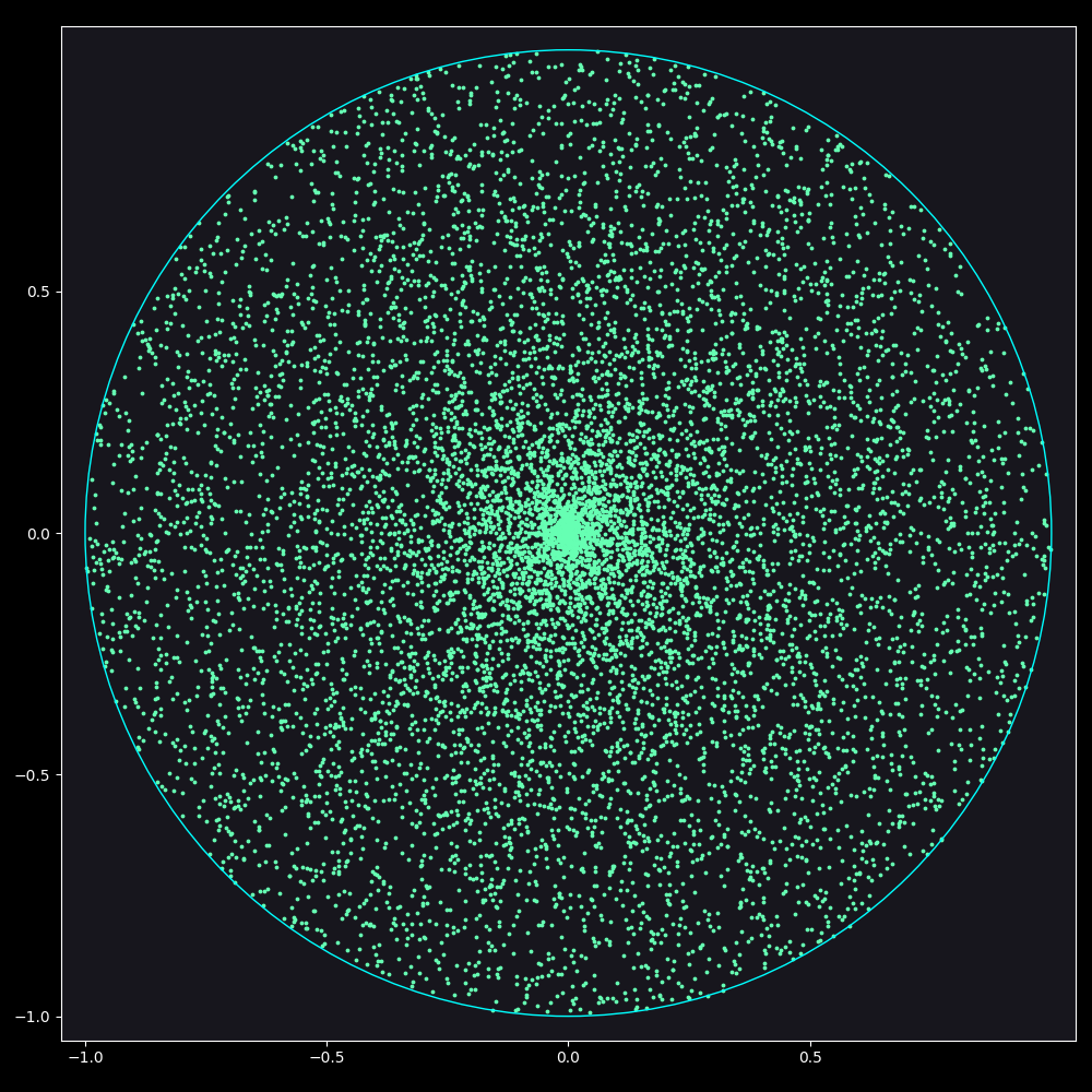
Figure 1: Naive Solution for Uniform distribution of points inside a circle
As can be seen, the points tend to cluster around the origin. But why is that the case? We have an equal chance of picking any radius when generating a point, so shouldn’t it distribute uniformly on all radii?
Clusterfix1
Let us simplify the ask and generate equally spaced points on circles of different radii first. As can be seen the smaller the radius the closer the points get. That is because points on the same circle can be at most $$inline-maths2R$$ away from each other.
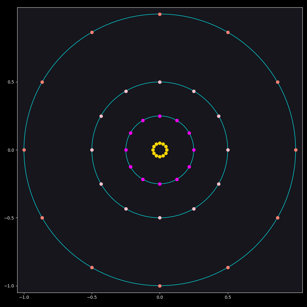
Figure 2: Equally Spaced Points on Circles of Different Radii
This means that the way we generate the random radii has to change. Currently we use an uniform distribution for it, meaning that any radius is just as likely as any other. But, as we have seen, this leads to clustering in the lower part of the distribution, so we need to choose a larger radius more times than a smaller one.
Therefore, the next question we need to answer is “how do we get this new distribution?”. We know that the larger the radius is the bigger the probability that it will be picked should be; because there is more “area”, in this case perimeter, that can be filled such that there is some minimum distance $$inline-mathsd$$ between all of them (see Figure 2 - difference between the smallest and biggest circle). We will start with the simplest form of modeling this, using direct proportionality ($$inline-mathsy=ax\Rightarrow{}y$$ $$inline-mathsis$$ $$inline-mathsdirectly$$ $$inline-mathsproportional$$ $$inline-mathsto$$ $$inline-mathsx$$).
Equations $$inline-maths(1)$$ to $$inline-maths(4)$$ model what we know already: that there is a function $$inline-mathsf(x)$$ $$inline-maths:$$ $$inline-maths[0,1]$$ $$inline-maths\rightarrow$$ $$inline-maths[0,1]$$ that models the distribution we want, that the sum of all (infinitely many) probabilities is $$inline-maths100\%$$ $$inline-maths=$$ $$inline-maths1$$, and that $$inline-mathsf(x)$$ is directly proportional to the circumference of the circle. Equation $$inline-maths(5)$$ codifies this in rigorous terms, here $$inline-mathsx$$ stands for the $$inline-maths2\pi{}R$$, and $$inline-mathsa$$ is the multiplier for the direct proportionality. Also notice that $$inline-mathsf(x)$$ is defined only on the $$inline-maths[0,1]$$ interval, because of the choices made in the introduction.
From equations $$inline-maths(2)$$ and $$inline-maths(5)$$ we can derive equation $$inline-maths(6)$$, which we solve to find the value of $$inline-mathsa$$ and get the formula for the probability density function (PDF).
Probability, Functions and Black Magic
Great, now that we have the PDF how do we sample it? Ideally there would be a way to just plug in the PDF into a black box and then use it to generate samples based on the PDF. Well, it just so happens that inverse transform sampling is such a black box. To use it, we must first calculate the cumulative distribution function (CDF) which tells us the probability that a sample from the PDF is smaller than the given value (see eq. $$inline-maths(7)$$). For a real-valued PDF, the CDF can be computed as the “sum” of the values of the PDF less than the given value, in this case, since the PDF is also continuous, the integral. The final step of the inverse transform sampling is to calculate the inverse of the CDF (ICDF), this will give us the black box function that, given a uniform distribution from 0 to 1 will convert it to the initial PDF.
Sufficiently Advanced Technology2
“Why and how does this work?”, I hear you ask. Well, the CDF produces a probability given a sample, and the ICDF produces a sample given a probability. The CDF calculates the probability that a new sample from the original PDF will be lower than a given number, and the ICDF calculates the number such that a new sample from the PDF has a given probability to be lower than it. In other words ICDF calculates the PDF sample whose CDF is the given probability. And since we use a uniform distribution to select that probability, meaning that all “probabilities” have an equal chance to be picked, it is almost like sampling the original PDF.
Figure 3 can be used to visualize why this is true. Using the ICDF is analogous to drawing horizontal lines and reflecting them down when it intersects the graph of the CDF. As can be seen from the figure, even though we sampled equally spaced points on the Y-axis, the result of the ICDF is that the points on the X-Axis cluster together the father away from 0 they get. This is consistent with the $$inline-mathsPDF=2x$$, which tells us that the larger the x is the more samples we should see around it.
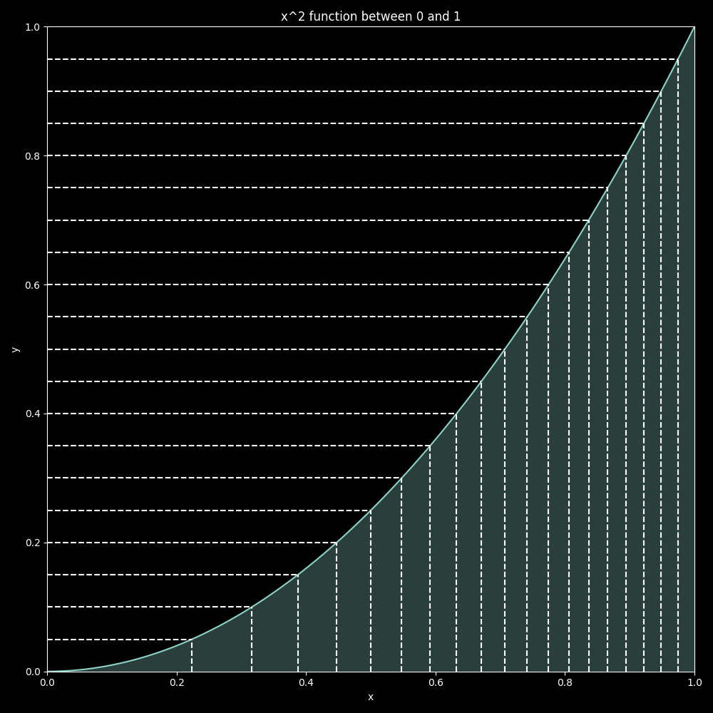
Figure 3: Plot of CDF
2Done
Now that we know how to sample the radius correctly it’s time to put it all together:
As can be seen in Figure 4 no obvious clustering is happening.
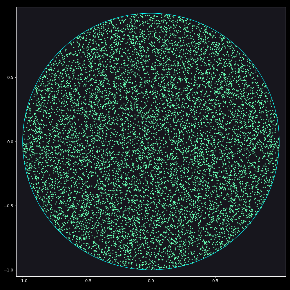
Figure 4: Proper Solution for Uniform distribution of points inside a circle
Going Even Further Beyond (3D)3
Now that we know how to sample points inside a circle, I won’t go over the naive approach for 3D (see Figure 5).
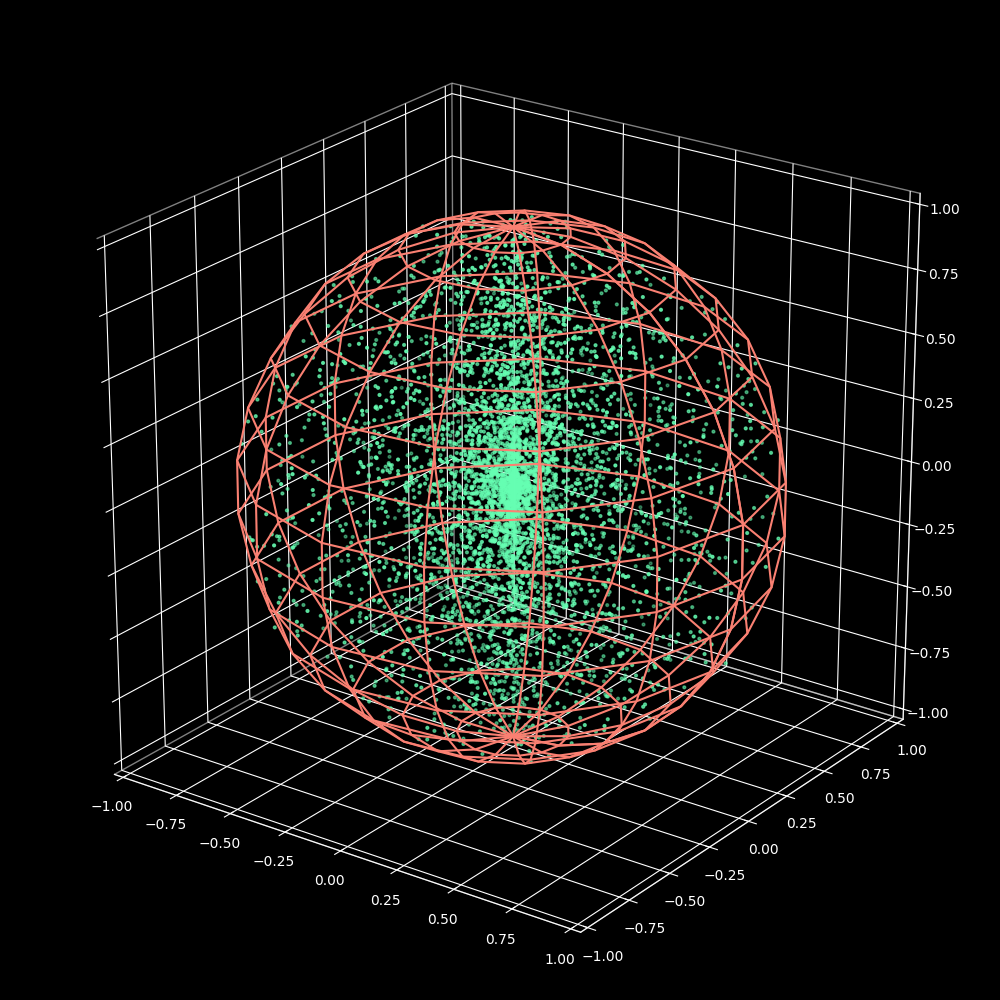
Figure 5: Naive Solution for Uniform distribution of points inside a sphere
Also we now have at least 2 methods of generating the points:
- “Split” the sphere into planes and generate points inside circles on those planes. (number of points needs to be scaled according to the radius of the circle)
- Generate points on the sphere and then scale the radius. (number of points needs to be scaled according to the radius of the sphere)
We will use #2 because I have already done the calculations for it, #1 is left as an exercise to the reader.
Next we need to choose a spherical coordinate system, for (in)convenience we will use:
- $$inline-mathsR\in[0;1]$$ = The radius of the sphere.
- $$inline-maths\theta\in[0;2\pi]$$ = angle around the
Zaxis measured form theXaxis. - $$inline-maths\phi\in[-\pi/2;\pi/2]$$ = angle between the vector from the origin to the point, and the plane
XY(see Figure 6, the $$inline-maths\phi$$ angle is represented by the cyan circle arc between the magenta line and theXYyellow plane).
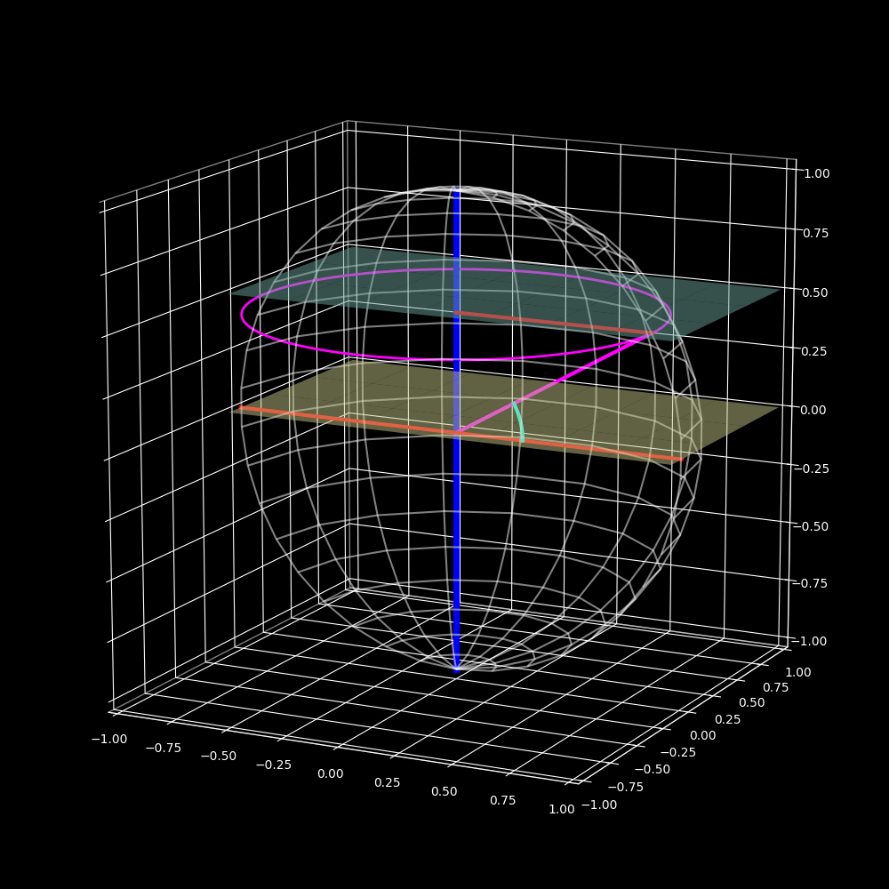
Figure 6: $$inline-maths\phi$$ angle visualization
Surface Level
To generate points on the sphere it is enough to know how to generate points on a circle (XY plane) and then vary the radius of the circle and the perpendicular axis (Z axis) component as well (in the range $$inline-maths[-R;R]$$). Using Figure 6 as reference, imagine moving the blue plane up and down; the magenta circle is the intersection between the blue plane and the sphere, notice that it’s radius is dependent on the height of the blue plane. Also notice that the height of the blue plane is dependent on the angle $$inline-maths\phi$$ and the radius of the sphere. Using a bit of trigonometry we get equation $$inline-maths(10)$$ that gives us a relationship between the radius of the sphere and the radius of the circle.
Next we will calculate a PDF for the probability of a point being on such a circle, depending on its radius. Equations $$inline-maths(11)$$ through $$inline-maths(16)$$ define this PDF. Start by assuming that the PDF is directly proportional to the circle perimeter, but since for this case $$inline-maths2\pi*R_{sphere}$$ is constant, the PDF is actually proportional only to $$inline-maths\cos(\phi)$$, the only variable part.
Next we use equations $$inline-maths(17)$$ through $$inline-maths(21)$$ to find $$inline-mathsa$$ (the proportionality factor) and the full definition of the PDF.
Next we calculate the CDF and ICDF (equations $$inline-maths(22)$$ through $$inline-maths(29)$$) so we can sample the distribution. The PDF depends on $$inline-maths\phi$$ which is defined in the range $$inline-maths[-\pi/2;\pi/2]$$, therefore so does the CDF.
Now putting all together we get the following formulas for generating points on a sphere of radius $$inline-mathsR$$.
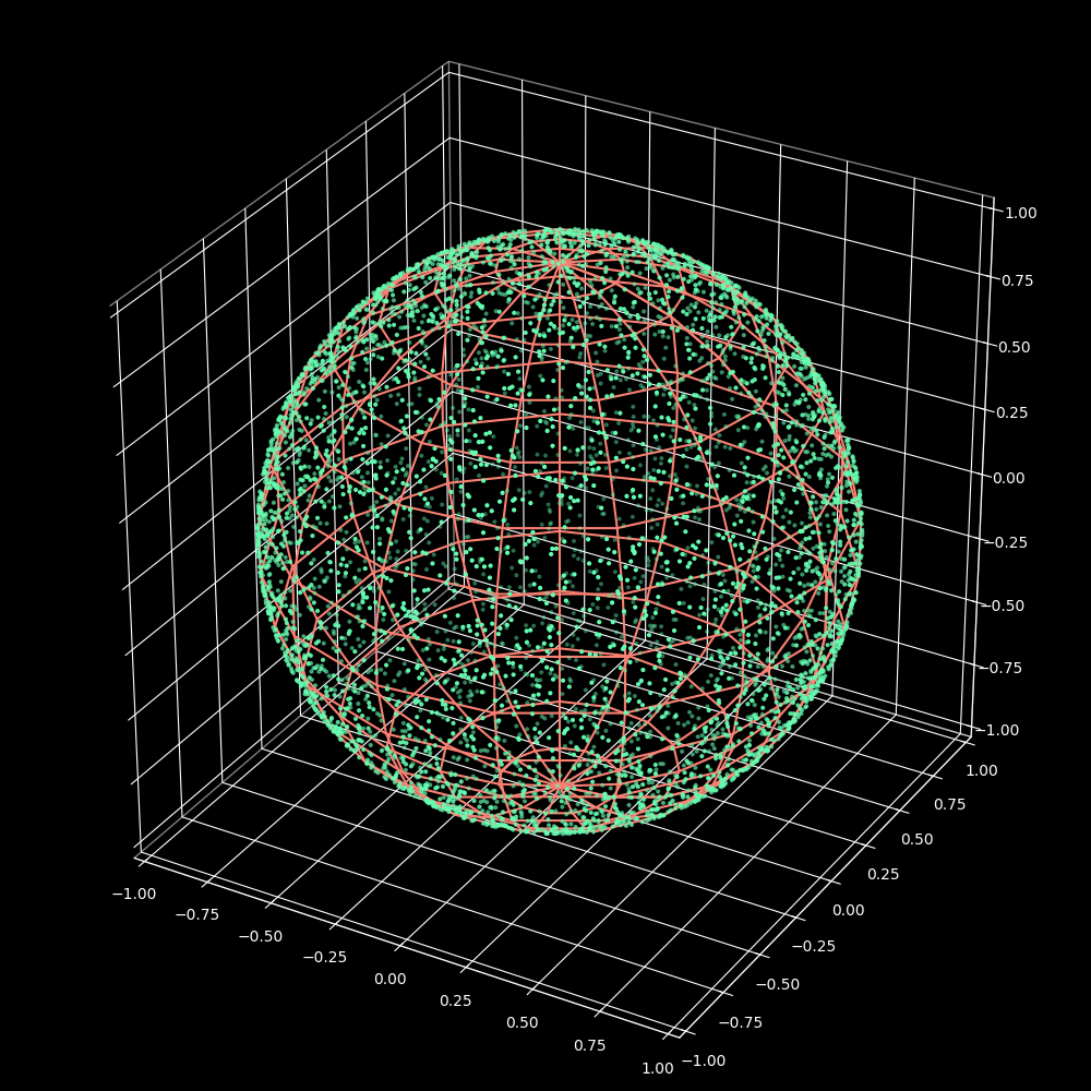
Figure 7: Uniform distribution of points on the surface of a sphere
Going Deeper
Now that we know how to generate points on a sphere all we have to do is vary the radius of the sphere we generate points on. But as we have already seen plenty of times, we need to be careful with the distribution of these radii (see Figure 2). So one last time with feeling: find the PDF ($$inline-maths(30)$$ to $$inline-maths(40)$$), compute the CDF ($$inline-maths(41)$$), compute ICDF ($$inline-maths(42)$$).
Using these we get the equations necessary to generate uniformly distributed points inside a sphere as such:
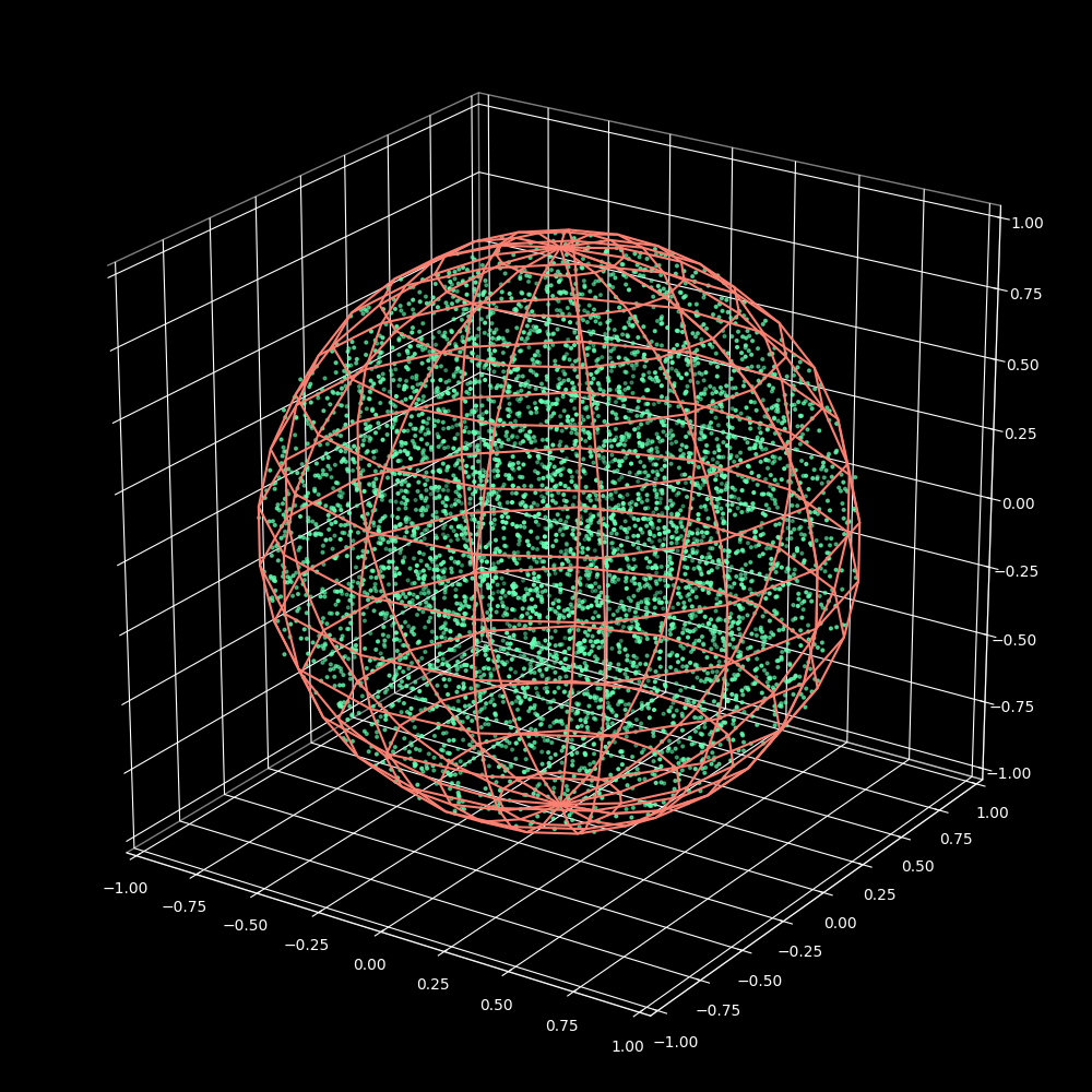
Figure 8: Proper Solution for Uniform distribution of points inside a sphere
Conclusion?
???
-
Opposite of clusterfuck. In this context it is used because of actively trying to solve a clustering issue. ↩︎
-
Reference to Arthur C. Clarke’s 3rd law: “Any sufficiently advanced technology is indistinguishable from magic.” ↩︎